Business Economics

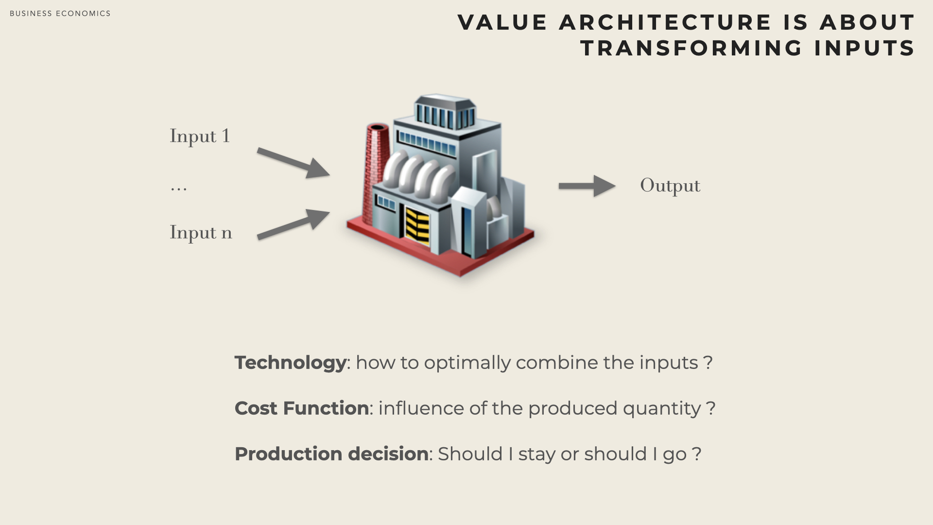
Economists call inputs factors and say that firm combine factors. They also represent the transformation as a so called production function. The function is characteristic of the technology (i.e. production processes) used. For a given production function, the output (and therefore the cost of producing the output) is a function of the various inputs.

Vertical Boundaries of the Firm

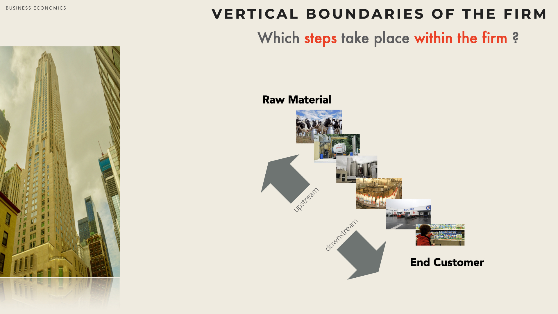
First, a firm needs to decide where it wants to operate along the Value System (or vertical chain). Any production process can be described as a sequence of stages (including inbound and outbound logistics, distribution and retailing) that flows from the raw inputs to the end customer.

« The production of any good or service usually requires many activities. The process that begins with the acquisition of raw materials and ends with the distribution & sale of finished goods and service is known as the vertical chain » [Besanko]

Note: Each stage can represent an industry in its own right, which is subject to specific competitive forces).

Within the production process, upstream activities are close to raw material and downstream activities to the end consumption.

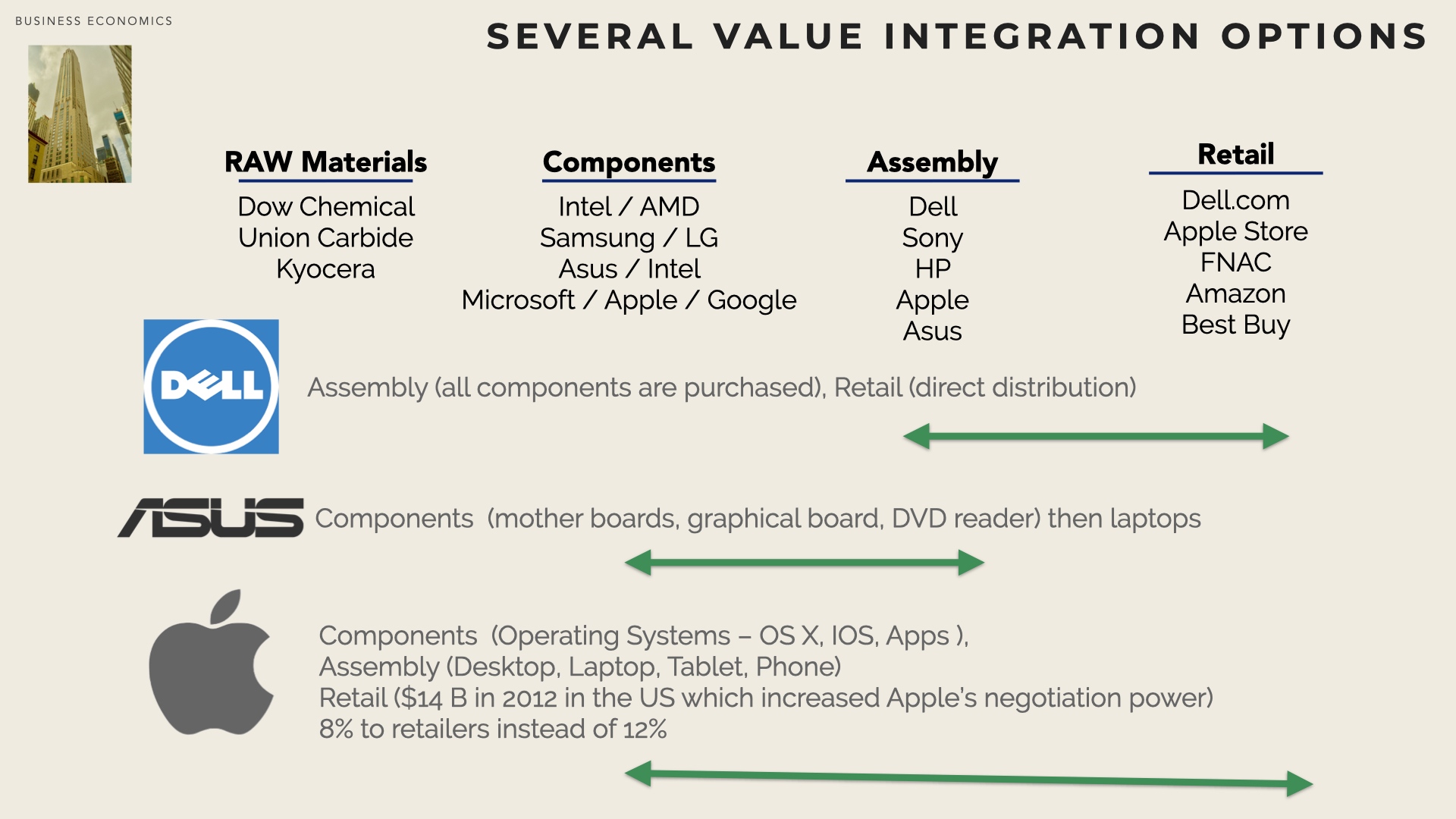
A firm that participates in more than one successive stage of the process is vertically integrated. Integration can be achieved through external growth (e.g. acquisition) or organic growth (green field development).

A backward integrated firm produces its own inputs whereas a forward integrated firm becomes its own ’customer’ (but there still should be some ’end customer’ at the end of the value chain). Integration can be hybrid in so that a firm may for instance decide to build some of its inputs while still relying on its suppliers for other inputs.

As an alternative to integration, a firm may decide to establish strategic alliances and/or tight contractual relationships with some upstream or downstream firms (e.g. franchise network). Such schemes are sometimes called quasi-integration.

When a firm decide to outsource some activities (i.e. purchase from the market) this is called vertical disintegration.

Notion of Value Chain

The concept of Value Chain was introduced by Porter ( [Porter85] ) in its seminal book. An internal value chain is the description of all the steps taken by the company to deliver the value proposition to their customer. It identifies the firm’s activities and their interaction. The model applies to one specific business (i.e. at business strategy level and not at corporate strategy level).

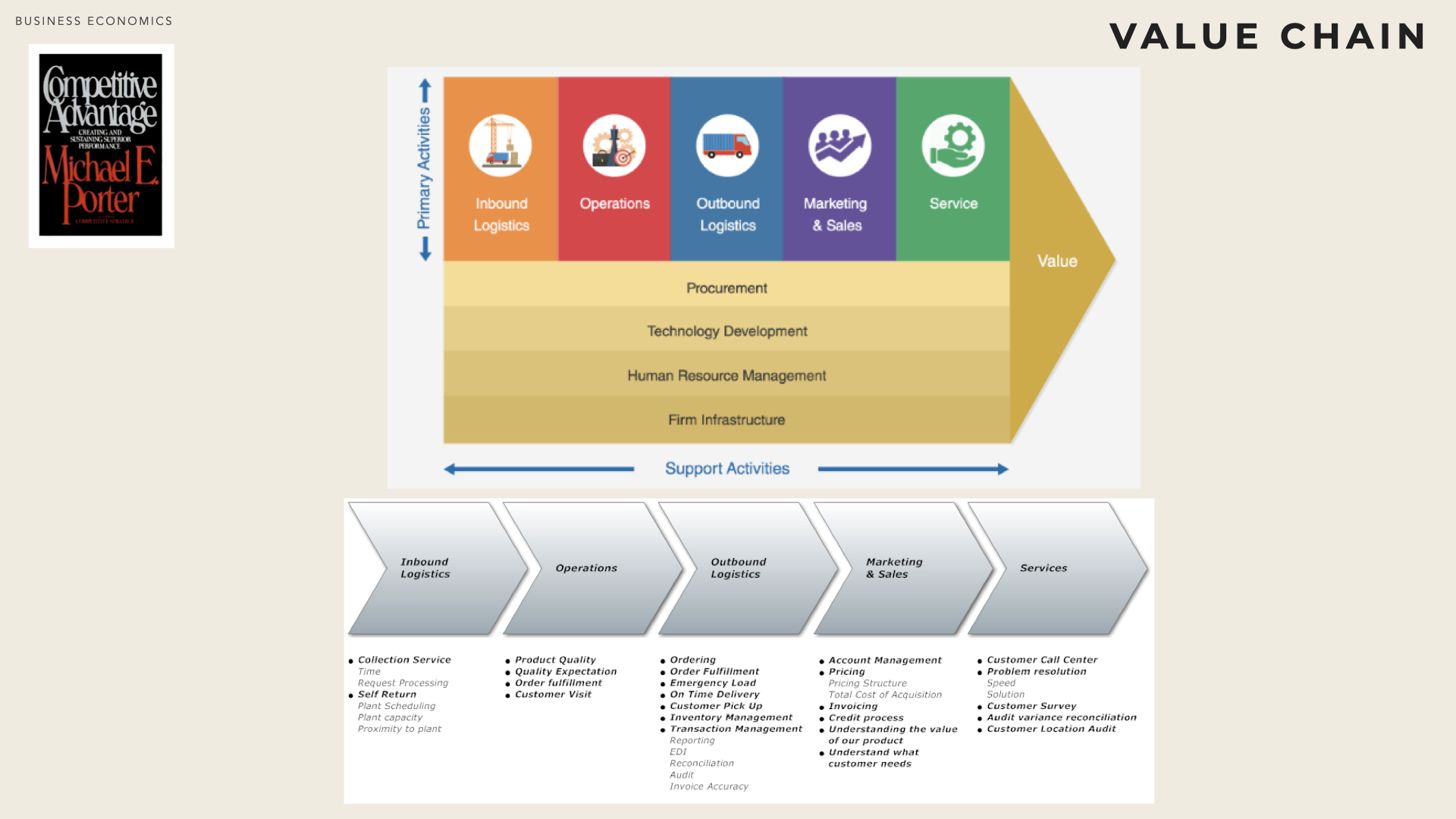
Classically activities are broken down into primary activities (directly adding value toward the output - i.e. that vary directly with the level of production) and support activities (that contribute indirectly to the output or are non adding any value to the product/services but are mandatory, for instance accounting).

The actual list of activities and the relevance of the categories are highly dependent on the type of business. For a multi-product firm (where support activities are shared among various business lines) the analysis can become tedious and allocating support costs to the various products can be very subjective.

However, when establishing a business case for a new product/service line, the value chain framework is a good framework to ensure that some activities are not neglected and/or some costs are not under-estimated.

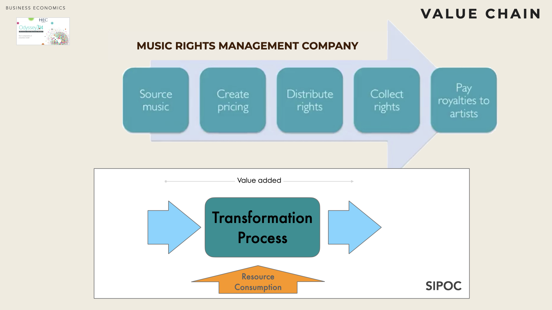
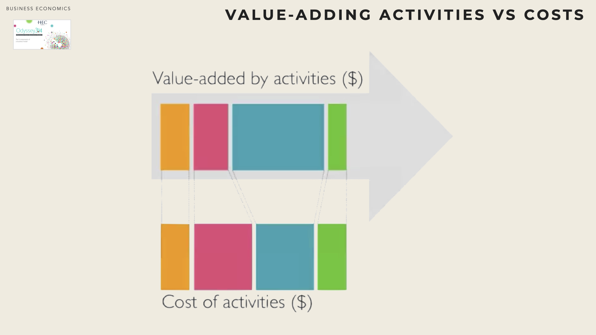
The value chain analysis is actually two-fold: i) delineate the sequence of activities and, ii) for each and activity, characterise how inputs are transformed and which resources are used / consumed in the process (cost structure and value addition to the customer).

Make vs Buy

The decision to rely on the market (buy from suppliers) or to produce internally (make) is often called a make vs buy decision.

A highly integrated firm performs most activities in-house. For instance, Benetton dyes fabrics, designs and assembles clothing, and operates retail stores [Besanko]. Other firms focus only on the design of their products while having already outsourced all their production.

By and large, a firm will decide to make (i.e. to produce internally) if it has the capability, the capacity and if it can produce at a cost equal or less than what the market can offer. Otherwise the firm would decide to buy.

It is noteworthy that Make vs Buy is not about deciding which production steps can be eliminated. Instead it is about deciding which steps should be performed in-house (or procure from suppliers) by the firm.

The external value chain describes how the business model of the company fits into a broader, sectoral logic. It underlines how the various players (suppliers, complementors) are contributing to value creation for customers. It may as well highlight which are the potential ways of improving the business model.

Classically several aspects must be taken into account before deciding to outsource activities:

• Does it solve a problem? although an obvious question, companies sometimes fail to identify the problems (e.g. capacity, cost, competence) that they are seeking to solve, before looking for an external provider.

• What degree of integration? with the other activities of the firm and how much is it contributing to the competitive advantage. Is the firm outsourcing activities or its complete business (which can be extremely risky).

• Will it improve performance? i.e.reduce costs, improve quality, shorten lead-time, increase higher reactivity, etc.

• Will it transform fixed costs into variable costs? reduce financial risks & capital expenditure, increase flexibility

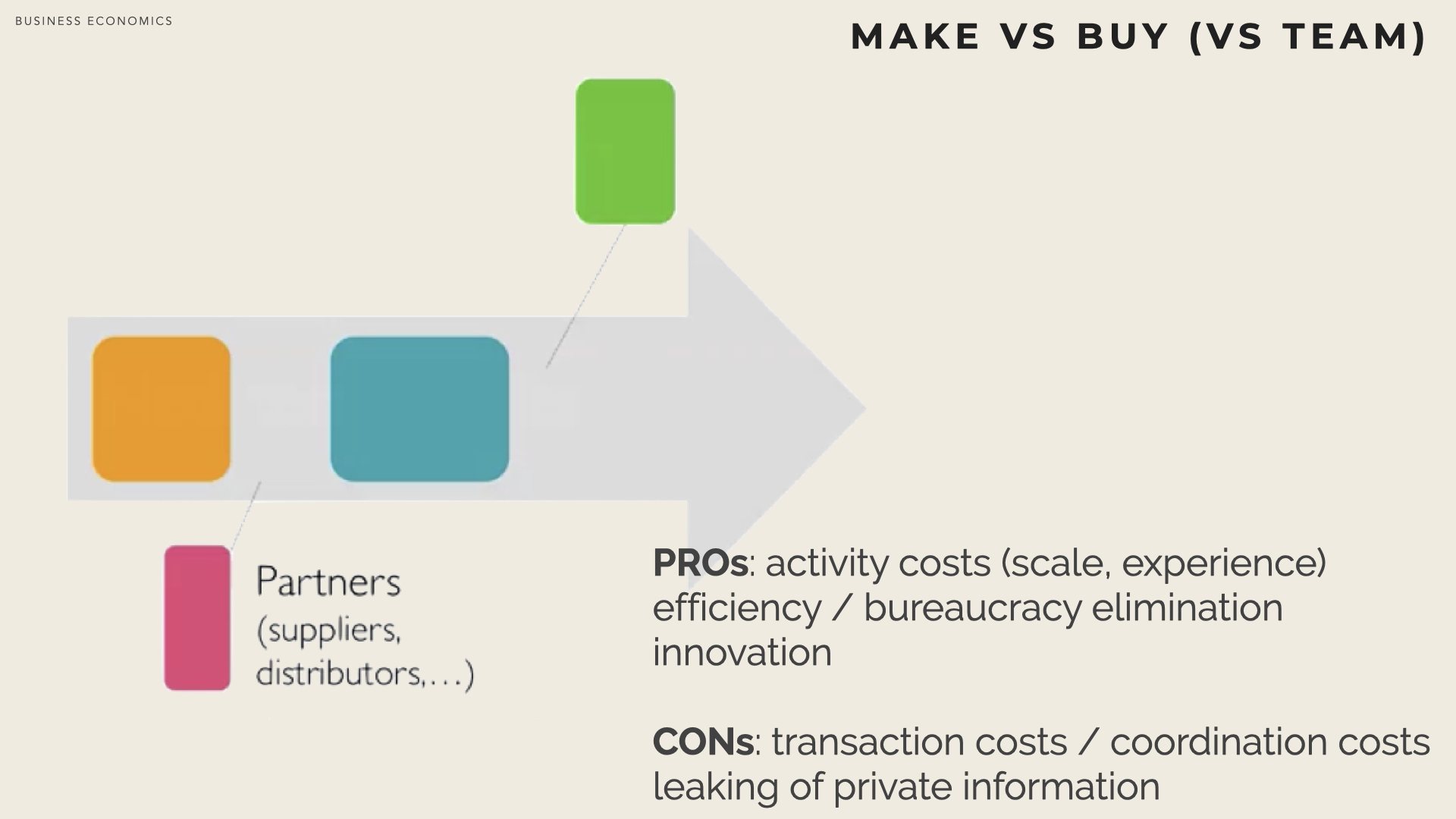
Choosing the market usually brings several benefits such as

• market firms can produce at a lower cost: i) as they aggregate the needs of many customers and serve a larger demand, they can achieve economies of scale (hence lower cost) that in-house production cannot, ii) being more specialized they can enjoy the experience effect earlier

• specialised market firms can be more innovative or simply control a set of skills & competence that are not available internally

• in a competitive market, firms seek to increase their efficiency and eliminate bureaucracy

However it may as well come with some drawbacks:

• Coordination costs (production flows from different sources) and risk of production flow disruption

• Transaction costs (see below)

• Leaking of private information (Intellectual property, forecast, etc…)

Frequent Make vs Buy Fallacies

make and buy are only options and there is a kind of continuum of options, between acquiring inputs on the spot from the market and building the inputs in-house.

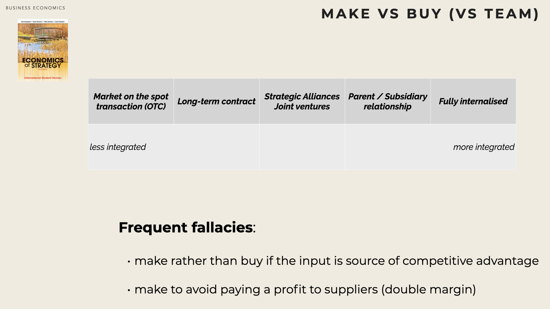
Make vs Buy is not black or White and there is a continuum between on the spot market access and full integration. Furthermore a firm may decide to insource some activities. This can be achieved organically or by acquiring one of the existing suppliers (or a firm that competes with the existing suppliers).

Firms should make rather than buy an input if that input is a source of competitive advantage. An input that can be (easily) acquired by any player from the market cannot be a source of competitive advantage.

Firms should make rather than buy to avoid paying a profit to a third party in other words, firm should backward integrate to capture the profit of its supplier. A Make or Buy decision must be looked at from the perspective of the firm and therefore the cost of making must be compared to the cost of purchasing (how much of that cost is captured as profit by the supplier is irrelevant).

Bureaucracy Effects

Although the term bureaucracy only appeared in the middle of the 18th century, it is associated with organized administrative systems that many forms of government have developed since 3500BC.

For strategists (and economists) however bureaucracy relates to control activities within a firm. It is often considered waste as i) it doesn’t directly contribute to the production process and ii) it is associated with conflict of interest, agency problems and influence costs.

Agency costs are the costs associated with i) shirking, ii) administrative audit and control and iii) deterrence measures to prevent shirking. A common way to limit shirking is to reward managers for the profit that their efforts contribute to the firm (bonus, stock options, etc…). However it is not always straightforward to evaluate such profit, even less for activities that are insulated from competition because they have captive internal customers.

Influence costs as Paul Milgrom and John Roberts ( [Milgrom90] ) call them, are another class of costs that often arise. The various departments or teams in a firm compete for funding, indeed there are often more ideas and requests than available budget. Managers will often seek to command more of their company’s resources to advance their career (and receive more personal reward), possibly at the expense of the company profit. To do so, manager may engage in a set of influence activities, including exaggerating the merits of their projects, badmouthing proposals from others, withholding information or key personnel. As a result of this asymmetry of information, resources (people, capital) are inefficiently allocated.

Transaction Costs

A complete contract stipulates each party’s rights and duties for each and every contingency that could happen during execution. It is very challenging to specify a complete contract as all potential contingencies must be identified and the associated course of actions for the two parties precisely defined.

In addition the required level of performance must be defined as well as means of measuring the actual performance during execution. Last but not least, the contract must be enforceable (for instance by a tribunal).

«Contracts list the set of tasks that each contracting party expects the other to perform and specify remedies in the event that one party doesn’t fulfill its obligations. If a firm could be certain that its partner would never shirk, there would be no reason for a contract.» [Besanko]

Most real-life contracts are incomplete (they don’t fully eliminate opportunities for shirking) mainly because i) it is non-realistic to identify all contingencies (even less for long-term contract), ii) it is very challenging to fully specify courses of actions and iii) very often the parties don’t have equal access to all information.

The concept of transactions cost was coined by Nobel prize winner R. Coase and initially disseminated by O. Williamson another Nobel Prize winner ( [Coase37] [Williamson81] ) . Coase stressed that if relying on the market was always more efficient than making within a firm, there would be no firm. He concluded that there must be some additional specific costs that are incurred when a firm buy from the market.

Williamson detailed what is encompassed into transaction costs: the time and expense of i) identifying suppliers, ii) seeking information, iii) negotiating, iv) writing and enforcing a contract as well as the costs incurred when suppliers exploit incomplete contracts to act opportunistically.

Incomplete contracting always entails some transaction costs, the largest part of which being the adverse consequence of opportunistic behavior and the costs of trying to prevent them.

A factor is said to be Relation-specific when it supports a particular contract and cannot be redeployed (or at a significant cost). For instance a manufacturing die (used to cut and shape material using a press) is both expensive and specific of the part being built. If a firm use an external design office and impose non-standard formats (e.g. software, methodology, unwritten routines) the corresponding skills and competence are relation-specific. Physical locations (e.g. factory or warehouse nearby the customer) are also relation-specific factors. Williamson stresses that once the parties have made a relation-specific investment a fundamental transformation unfolds and the relationship evolves from “many options” bargaining situation to “limited or single option”.

The relation-specific investment is the portion of the investment that cannot be recovered in case the contract doesn’t materialise. The quasi-rent is the extra profit derived from the materialisation of the contract compared to the next-best alternative once the investment is made. When an asset is specific, the quasi-rent is strictly positive (i.e. the next-best alternative is not as good as the contract materialisation). At the extreme, the investment is so specific that the quasi-rent is the full profit of the contract.

Holdup problem if the quasi-rent is substantial (i.e. the supplier has a lot to lose), the customer may be tempted to exploit in one way or another breaches in the contract and renegotiate at a lower price once the investment is made.

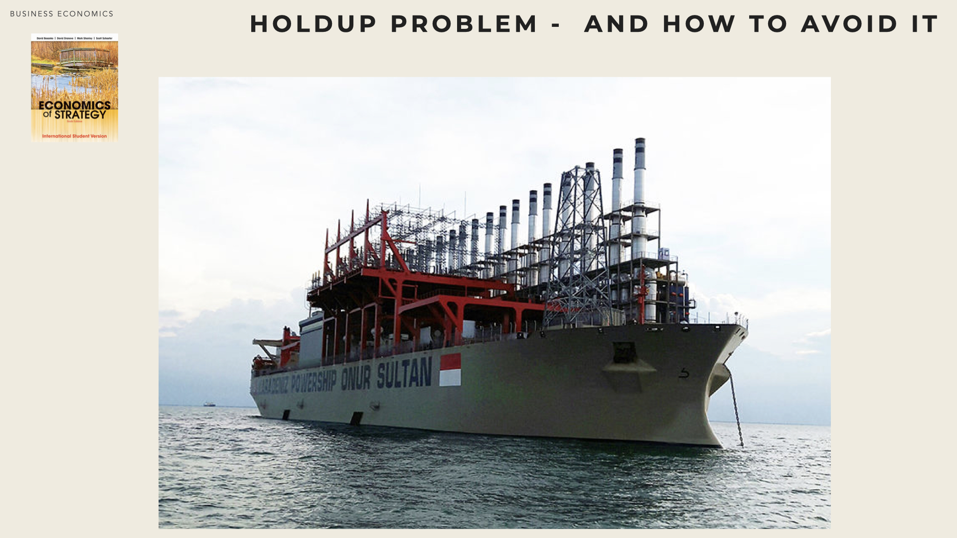
Power plants are highly specialised assets. To avoid the hold-up problem (in developing countries), power plants are built on floating barges, thereby the geographic specificity can be partially eliminated and if a government defaults or seeks to leverage opportunistic behaviours, the power plant can be relocalised elsewhere at low cost. [Besanko]

Why seeking to vertically integrate ?

Vertical integration can be driven by several reasons:

• Transaction Costs a firm incurs costs besides the price when trading with other (e.g. searching and assessing potential suppliers, running selections, writing and enforcing contracts). A firm that vertically integrate avoids such costs (however it incurs new management and control costs).

• Avoid opportunistic behaviour it can be very difficult and costly to anticipate all potential situations in a contract. Therefore there is a risk that one of the parties may want to take advantage of the other if the circumstances permit. Usually the solution consists in signing long-term agreements, where most of the attributes of the relationship are clearly specified. However when the risk of opportunistic behavior is too high (for instance when a firm only deal with one other firm), integration is preferable to any commercial relationships.

• Asymmetry of information when one firm owns private knowledge that can’t be taken into account when the contract is established, that firm is likely to seek taking advantage of the less knowledgeable firm. If the buyer anticipates the asymmetry, it will increase monitoring and will therefore incur additional costs.

• Control quality and ensure steady supply when a supplier deliver components that are crucial, are difficult to store or represent high unit price, the buyer will try to control production. Alternatively, the buyer may decide to integrate its key suppliers and take full responsibility for the supply.

• Avoiding regulation /Anti-trust firms may also vertically integrate to avoid government price controls, taxes, and regulations. A vertically integrated firm avoids price controls by selling to itself (internal transaction). Firms also integrate to lower their taxes. Tax rates vary by country, state, and type of product. A vertically integrated firm can shift profits from one of its operations to another simply by changing the transfer price at which it sells its internally produced materials from one division to another.

• Eliminating Market Power a firm that faces direct suppliers or retailers that are too strong may try to either foster competition (even sometimes create competitors) or eliminate that market power by vertically integrating.

Property Rights of the Firm

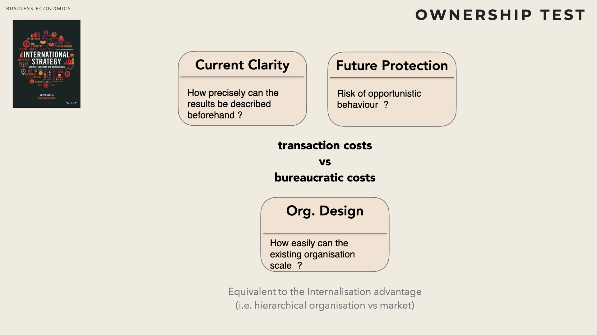
Integration allows the firm to control resources, costs and profit when contract are incomplete and partners would disagree. When contracts are complete it doesn’t matter who own the assets.

According to Oliver Hart, Sanford Grossman and John Moore: « Integration determines the ownership and control of assets, and it is through ownership and control that firms are able to exploit contractual incompleteness. »

If a firm rely on a partner’s asset, it will have to persuade the partner to cooperate (or to execute the contract). By contrast, if the firm owns the asset it can decide (residual rights of control) how to use that asset as new opportunities unfold.

Horizontal Boundaries of the Firm

The Horizontal boundaries correspond to the quantity (and variety) of product sold by a single firm. The horizontal boundaries can be measured in market share. Economies of scale, scope and experience allow some firm to derive of cost advantage that can translate either in lower price or higher profit.

Horizontal boundaries must be understood within a segment of the Value system (i.e. within one given industry). It mainly relates to the size of a company and how much market share it controls.

A firm can expand its horizontal boundaries through organic growth (increasing its production level / sales) or through acquisition of firms operating in the same industry. The principal benefit of engaging in horizontal integration is that i) it eliminates competition from other firms and ii) it allows to increase economies of scale (when applicable) and reduce the average unit costs.

Economics 101

This is only a brief introduction. The interested reader should turn to reference books such as ( ( [Besanko13] [Pindyck12] [Mas-Colell95] [Varian14] ) )

Total costs, fixed costs, variable costs
The total cost \( TC \) of producing a quantity \( q \) (considered as a flow i.e. production of a certain quantity in a given period of time – usually a year or a month) is the sum of fixed costs \( FC \) which don’t depend on \( q \) and variable costs \( VC \) which is a function of \( q \).

\[ TC(q) = FC + VC(q) \]

Note: \(VC(q)\) is the cost of producing \(q\) units (and not the unitary cost when the level of production is \(q\).

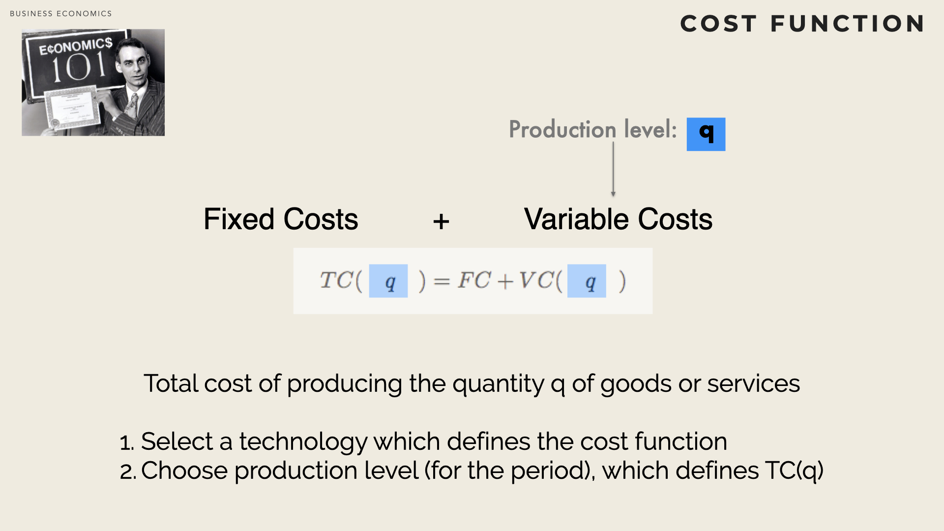
It is noteworthy that the notion of fixed vs variable depends on the considered time horizon. In the very short term most costs are fixed (as a firm can usually not react instantaneously to changes) and by contrast in the very long run all costs are variable (a firm may decide to sell existing fixed assets or on the contrary to acquire additional ones). Usually we consider that i) a firm commits to a production technology, tooling and facilities (fixed costs) with a maximum output level and ii) the firm can adjust its production level (variable costs) within these boundaries.

• Selecting a technology induces a total cost function. Two different technologies (i.e. two different ways to produce the same outputs) will usually have different fixed and variable costs.

• Selecting a production level determines the average cost. For a given production level, the notion of average costs helps comparing the two.

Average costs
The average cost \( AC \) is the total cost (at a given level of production) divided by the quantity produced.

\[ AC(q) = \frac{TC(q)}{q} = \frac{FC + VC(q)}{q} \]

Why is this notion important? Because it provides a per-unit-cost. In other words, knowing that the production level is \( Q \), then we can consider that it costs \( n.AC(Q) \) to the firm to produce \( n \) pieces of output (don’t confuse \(n\) the number of costed units with \(Q\), the total production level ).

\( AC \) is usually not constant (i.e. it depends on \(Q\) the total quantity produced). The average cost curve is usually U-Shaped (although it can also be L-Shaped).

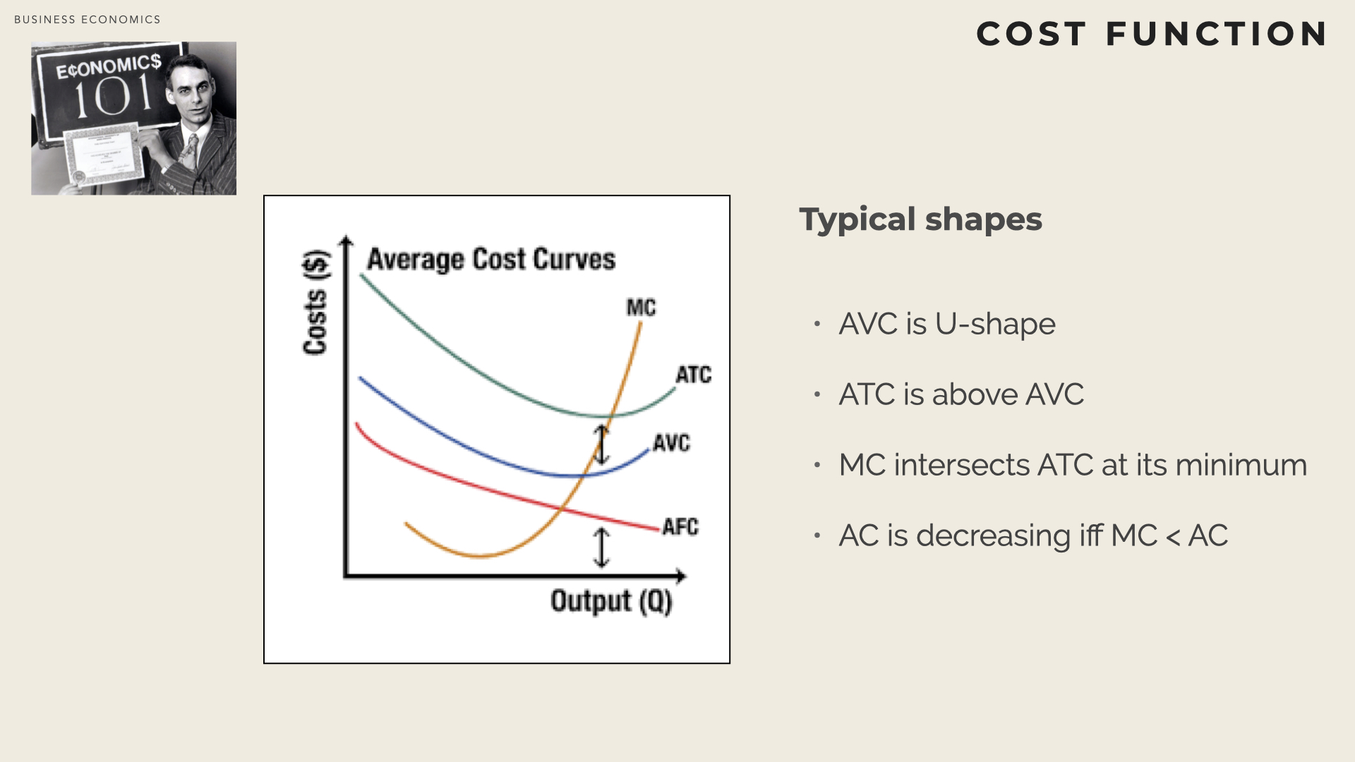
In many industries, the average cost tend to decrease with production volume. This is for instance, the case when fix costs are high relative to variable costs (the amortisation of fix costs can be spread over more units). When the production level reaches a certain threshold, the average cost remains stable over a production range and starts to increase again above a certain level.

Marginal costs
The marginal cost (at a given production level) is the incremental cost of producing one additional unit.

\[ MC(q) = \frac{TC(q + \Delta q) - TC(q) }{ \Delta(q)} = - \frac{FC + VC(q +\Delta q) - FC - VC(q) )}{\Delta q} = \frac{ VC(q +\Delta q) - VC(q) )}{\Delta q}\]

In other words, \( MC \) is the derivative of \( TC \) as well as \( VC \) (\( FC \) being a constant, its derivative is null).

\[ MC(q) = \frac{d TC(q)}{dq} = \frac{d VC(q) }{ dq} \]

The derivative of the Average cost is

\[ \frac{dAC(q)}{dq} = -\frac{F+VC(q)}{q^2} + \frac{1}{q}.\frac{dV(q)}{dq} \] which can be rewritten:

\[ \frac{dAC(q)}{dq} = \frac{1}{q} (\frac{dV(q)}{dq} -AC(q)) = \frac{MC(q) - AC(q) }{q} \]

When the marginal costs is lower than the average cost, the average cost curve is decreasing. When the marginal cost equals the average cost the average cost curve is flat (and at its lowest value) and when the marginal cost is higher than the average cost, the curve is increasing.

The optimum corresponds to \( AC(q) = MC(q) \).

Economies of Scale

In many industries, average unit costs tend to decrease with the production volume (at least until a certain production threshold). This is for instance the case when the fixed costs are high relative to variable costs (the amortization of fixed costs can be spread over more units).

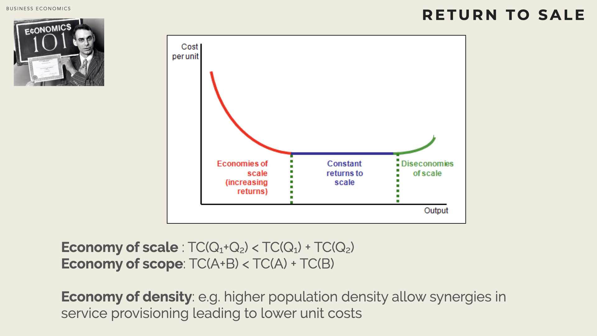
The production process for a specific good or service exhibits economies of scale over a range of output when average cost (i.e. cost per unit of output) declines over that range.

Informally when there are economies of scale and scope bigger is better [Besanko]

The area where marginal costs (the incremental costs of producing one more item) are less than average costs brings up economies of scale (aka increasing returns). A firm has a strong incentive to increase its production level within the area of increasing returns (the higher the production level, the lower the unit costs).

The smallest quantity for which economies of scale are exhausted (i.e. where the constant return area starts ) is named the minimum efficient scale

However, if the firm continues to increase its production level, sooner or later it will hit the area of decreasing returns and starts to generate diseconomies of scale (for instance because the new production level would require an additional facility which would increase fix costs).

Multi-business firms may enjoy economies of scope when some inputs (procured parts, production activities) are used for several pro- ducts. In such a case the cumulated production (of all such products) is taken into account to compute unit costs (average total cost per unit).

The existence of economies of scope between two different businesses may underpin some corporate advantage. Owning the two businesses creates value in addition to the intrinsic value of each business taken in isolation.

When an average cost curve is L-shaped, costs decrease up to the minimum efficient scale of production and remain stable beyond.

Example with linear variable costs
Let’s assume that the variable cost is a linear function, i.e. \( VC(q) = a.q \).

The total cost is \( TC(q) = FC + a.q \) and the average cost is \( AC(q) = \frac{FC}{q} + a \).

The bigger the quantity \( q \) produced, the smaller the average cost (for an infinite quantity \( AC(q) \approx a\))

In that case, the marginal cost is constant \( MC(q) = \frac{VC(q)}{q} = a \) and the average cost is always decreasing. The average costs decreases when q increases as the fix part becomes more and more diluted.

Example with more complex variable costs
This time let’s assume that the variable cost is a more complex function \( VC(q) = a.q + b.q^2 \). There is still a linear part but also a quadratic element \( bq^2\).

The total cost is \( TC(q) = FC + a.q + b.q^2 \) and the average cost is \( AC(q) = \frac{FC}{q} + a + b.q \). The marginal cost is \( MC(q) = a + 2b. q \).

The optimum corresponds to:

\( AC(q) = MC(q) \)

i.e. \( \frac{FC}{q} + a + b.q = a + 2b.q\)

i.e. \( \frac{FC}{q} = b.q\)

i.e. \( q_0 = \sqrt{\frac{FC}{b}}\)

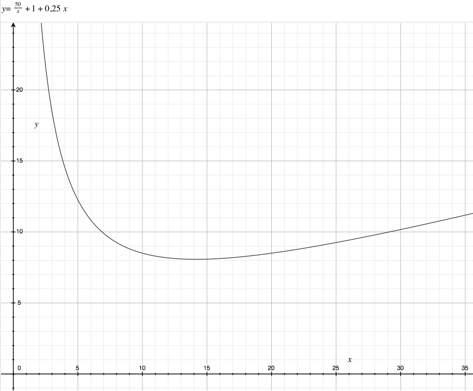
The average cost decreases until the quantity reaches \( q_0 \) and then starts to grow.

Reasons for economies of scale

• Spreading of fixed costs fixed costs derive from factors cannot be scaled down below a certain size (e.g. factories, machine). Fixed-costs also include Advertising, Research & Development costs and set-up costs (i.e. expenditures before any revenues). In many production processes, production capacity is proportional to the volume whereas total cost is proportional to the surface area.

• Economies of density arise when the number of customers increase in a geographic area. Economies of density also applies to all kind of network (telecommunication, airline hub, digital platform).

• Purchasing Power most suppliers give discounts based on quantities purchased

• Inventories firms carry inventory to mitigate the risk of production disruption (e.g. despite a machine being out of service, the full process must continue to run while the machine is being repaired). The higher the production level, the lower the ratio of inventory (law of big numbers).

Reasons for diseconomies of scale

• Increasing production (aka production rate) usually is not without problem. As the machines are more loaded they are more prone to failures which disrupts production and entails additional costs (non quality, scrapping, additional lead time, …). More workers also means that more people are needed to coordinate, plan and lead (i.e. additional overhead, bureaucracy costs).

• When production continues to grow, the fixed assets (e.g. machinery, plants, warehouses, …) will reach their limit. Increasing any further production will require increasing capacity and therefore fixed costs.

• Labor Cost usually grows with larger firms as they usually offer higher compensation and benefits (wages, bonuses, work council). However it is noteworthy that worker turnover is often lower at larger firms (which reduces the one-off costs of hiring and training new recruits).

Economies of Scope

The total cost of producing simultaneously \( X \) and \( Y \) is less than the cumulative cost of producing the two procuts separately.

\( TC(Q_x, Q_y) < TC(Q_x,0) + TC(0, Q_y) \)

Experience curve

In many industries, significant productivity efficiency and improvement are gained with the cumulated level of production. Please note that economies of scale are driven by the level of production within a period (typically the year) whereas the experience effect is linked to the cumulated production level (independently of any time reference).

The effect experience can be due to several factors:

• Labour efficiency (learning by doing, getting more confident, etc)

• Standardisation, method & process improvement

• Better automation, product redesign

In industries where the experience effect is important (for a typical firm, doubling cumulative output reduces average costs by 20%), players will seek to reach the highest cumulated production as quick as they can. They will therefore try to extend their market shares. A firm that can significantly benefit from learning, will often ramp-up production faster to gain from experience quicker.

When growth is limited, the industry structure becomes rigid (zero sum games between the players). Players will therefore seek to benefit as much as they can from any market growth (e.g. acquiring new market shares) so that they are in the most favourable situation (cost-wise) when market gets rigid. This is even more crucial in industries where products are highly standardised (commoditisation) where price is the only source of differentiation.

Experience effect equation
Bruce Henderson (who founded the Boston Consulting Group) had noted that the relative decrease of certain variable costs was proportional to the relative increase in cumulated production – in other words the decrease of costs in percentage is proportional to the increase in percentage of the cumulated production.

\[ \frac{\Delta C(q)}{C(q)} = -k . \frac{ \Delta q}{q} \]

This is equivalent to say that when the production doubles ( \( \Delta q = 2 q \) ), the variable cost is divided by a constant factor ( \( \Delta C(q) = -2k. C(q) \) ).

This relationship was probably first quantified in 1936 at Wright-Patterson Air Force Base in the United States, where it was determined that every time total aircraft production doubled, the required labour time decreased by 10 to 15 percent. Subsequent empirical studies from other industries have yielded different values ranging from only a couple of percentages up to 30%, but in most cases it is a constant percentage: It did not vary at different scales of operation. The Learning Curve model posits that for each doubling of the total quantity of items produced, costs decrease by a fixed proportion. [wikipedia]

The experience effect is represented by the differential equation: \( \frac{ dC(q)}{C(q)} = -k . \frac{ dq}{q} \), can be solved as \( ln(C(q)) = -kln(q) + C_0 \).

This then gives \( C(q) = \alpha . q^{-k} \).

If \( q = n \), the cost of producing the nth unit is \( C_n = \alpha . n^{-k} \).

As \( C_n = \alpha . 1^{-k} = \alpha \), then

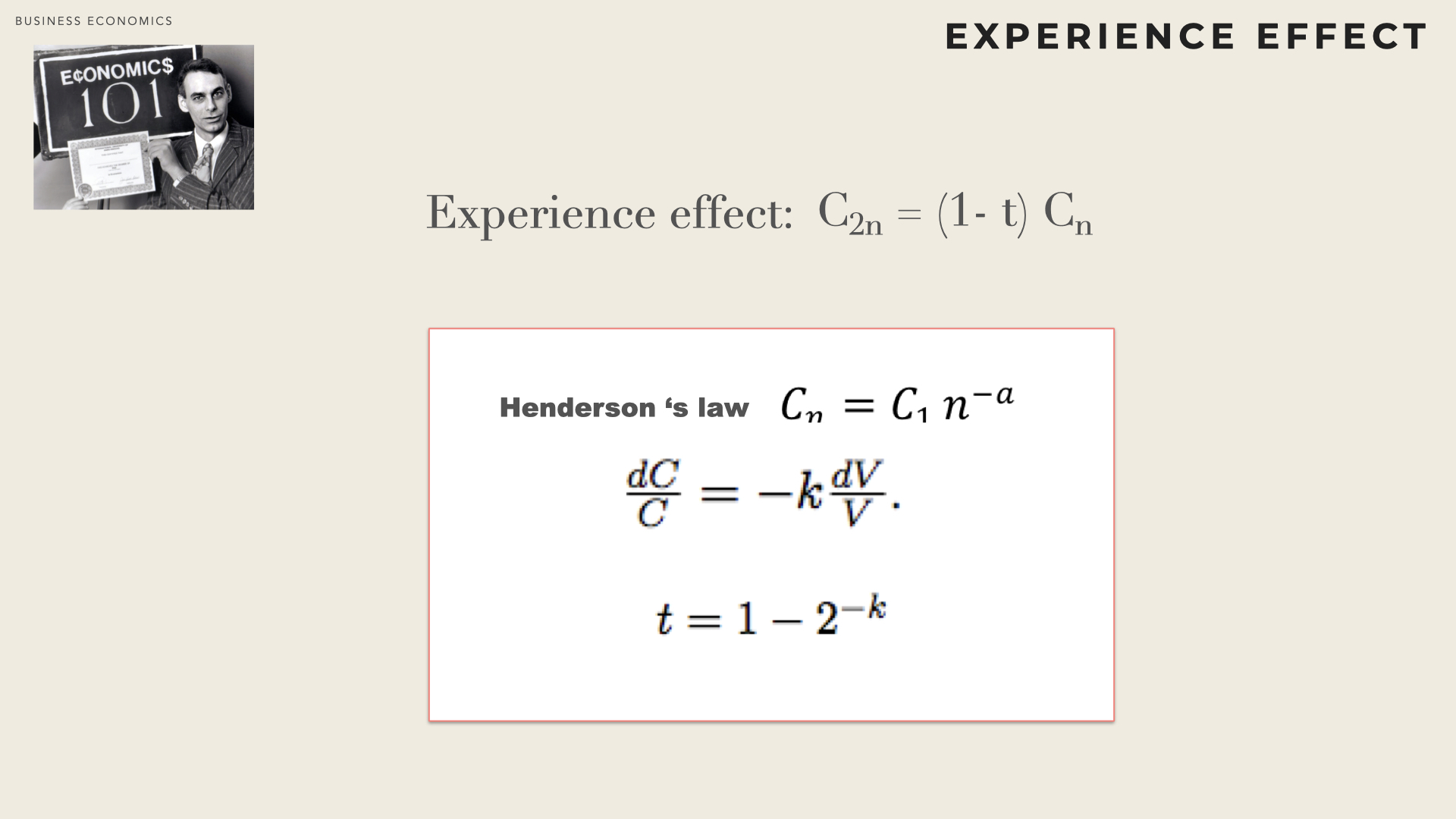
\[ C_n = C_1 . n^{-k} \]

The unit costs of the nth unit is linked to the unit costs of the first unit. k is a constant (elasticity of costs with regard to output), specific of the industry. One can check that when the cumulated production doubles \( C_{2n} = C_1 .(2n)^{-k} = C_1n^{-k}. 2^{-k} = C_n. 2^{-k}\).

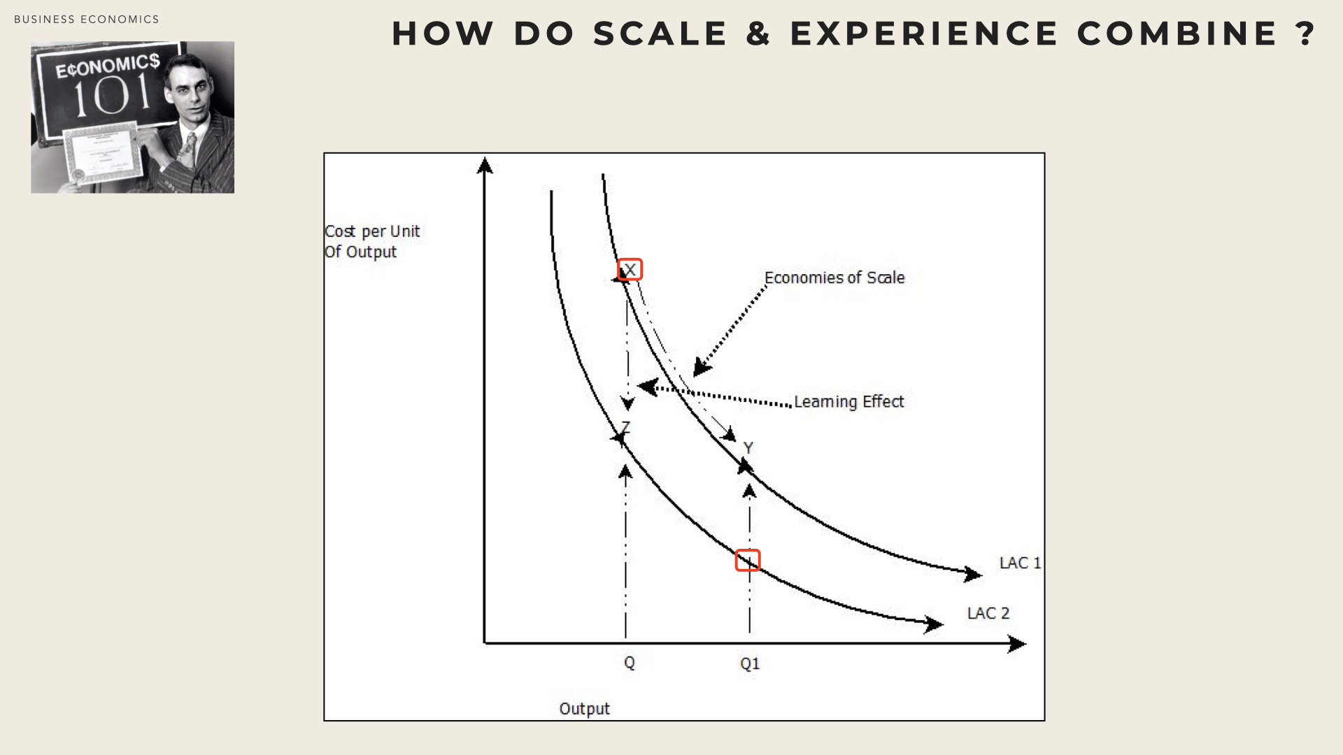
Combining Learning Effect and Economies of scale
When economies of scale are absent (or when a firm operate beyond the minimum efficient threshold) the average cost function is an horizontal line ( \( AC(q) = AC_1 \)). The experience effect can shit the average cost function. For instance when the cumulative production doubles then the average cost function becomes an other horizontal line ( \( AC(q) = AC_2 \) with \( AC_1 < AC_2 \) ).

The Five-Forces Framework

This famous framework ( [Porter79] [Porter08a] ) is a tool to analyse the structure of an industry, to describe the intensity of competition and to understand the origin of its long-term profitability level. Porter’s decisive contribution with the Five-Forces framework is in recognising profitability is not only influenced by the rivalry between direct competitors.

The objective of the analysis is therefore two-fold : on the one hand it delineates the industry and points out its dynamic (what are the long-run performance drivers); on the other, it pinpoints the “forces” that most influence the profitability so that an industry player can seek to fight against these forces and/or shape them to its advantage

A 5-Forces analysis will typically seek to address aspects such as :

• what industries to enter (respectively to exit) ?

• what influence can be exerted ?

• How are competitors differently affected by changes in the industry (e.g. raising barriers by increasing investment spending)

More technically, industries can be defined as groups of firms with low cross-price elasticity: i.e. price evolution within one group has small or no impact on the demand for goods in the other groups. For instance, an increase in coffee price does not affect postal services prices.

According to Porter, the configuration of the five forces is specific to each industry and rather stable over time.

Market Definition

« One cannot analyze competition without first identifying the competitors and competitors are the firms whose strategic choices directly affect one another.» ( [Besanko13] )

Antitrust agencies such as the DoJ (Department of Justice) in the US, the EC (European Commission) in the EU or the JFTC (Japan Fair Trade Commission) seek to limit anticompetitive conducts and to prevent situations where firms might abuse their market power.

Besanko provides the example of an hypothetical merger between Audi and Mercedes. Defining the market as German Luxury Cars would limit the players to Audi, Mercedes & BMW. A merger between two of these players would translate into significant market concentration (it would reduce the number of players to 2, down from 3). However, if the market is defined as All luxury cars additional players such as Lexus, Infiniti, Jaguar should be considered as well. The SSNIP provides means to determine which market definition is the closest to reality. If by merging, Audi and Mercedes could raise their prices by at least 5% then it would be the sign that they face little competition from non-German brands, otherwise the larger market definition applies.

The Five forces

Barney ( [Barney91] ) underlines that the market-view of the firm focuses on competitive imperfections in product markets to explain persistent differences in firm performance.

The 5-forces framework is one of the most prominent tools to underline such imperfection and identify opportunities to earn superior returns. However, whether a firm can gain a competitive advantage doesn’t depend solely on strategies that create competitive imperfections in product markets but as well on the total cost of implementing these strategies (which is determined by the competitiveness of the strategic factors).

This section mainly draws from Porter’s articles.

The Five Forces Framework ( [Porter79] [Porter08a] ) is a tool to analyse the structure of an industry, that is to describe the intensity of competition and to understand the origin of its long-term profitability level.

«With the ‘Five Forces’, my goal has been to develop rigorous and useful frameworks that efficiently bridge the gap between theory and practice » – [Porter, 2008b].

Porter’s decisive contribution with the Five-Forces framework is in recognising profitability is not only influenced by the rivalry between direct competitors. According to him, the configuration of the five forces is specific to each industry. The objective of the analysis is therefore two-fold: i) it delineates the industry and points out its dynamic (what are the long-run performance drivers) and ii) it pinpoints the “forces” that most influence the profitability so that an industry player can seek to fight against these forces and/or shape them to its advantage.

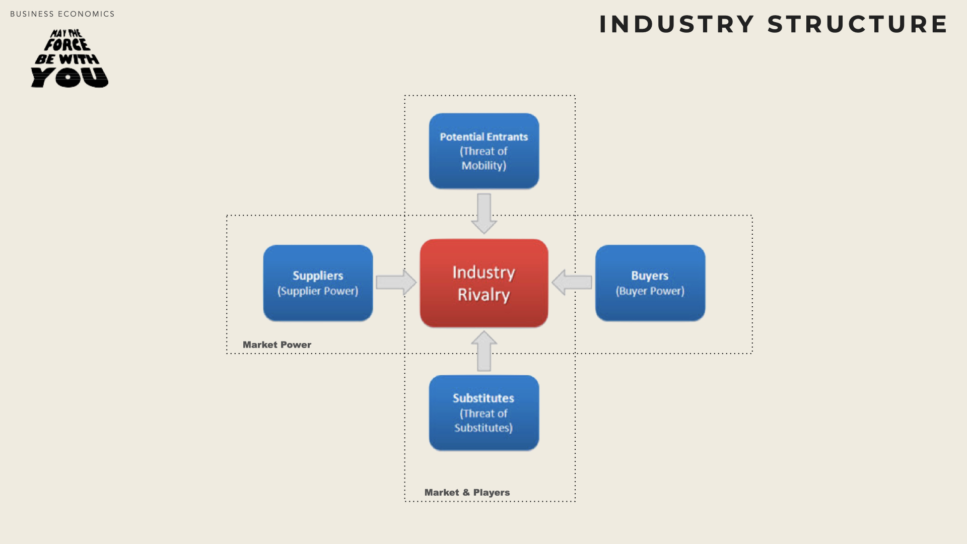
«In essence, the job of the strategist is to understand and cope with competition. Competition for profits goes beyond established industry rivals to include four other competitive forces as well : customers, suppliers, potential entrants and substitute products. The extended rivalry that results from all five forces defines an industry’s structure and shapes the nature of competitive interaction within an industry. […] The point of industry analysis is not to declare the industry attractive or unattractive but to understand the underpinning s of competition and root cause of profitability » – [Porter,1979].

Companies in the competitive field should not be defined in terms of product types, but rather in terms of the customers needs they served. This encourages decision maker to more precisely identify new entrant / substitutes and as well broaden the potential growth opportunities spectrum.

Intense forces will tend to reduce industry profitability and no firm will earn attractive returns. By contrast, when forces are softer, players can generate profit in excess to their cost of capital. The five forces framework helps assessing the market Power.

An industry analysis should include quantitative elements as much as possible: „the effects of the forces are directly tied to the income statements and balance sheet of industry participants” ([Porter, 1998]). The analysis should not be limited to drawing the static picture of current forces but should also seek to anticipate shifts in each force and forecast how it might trigger reactions in the other.

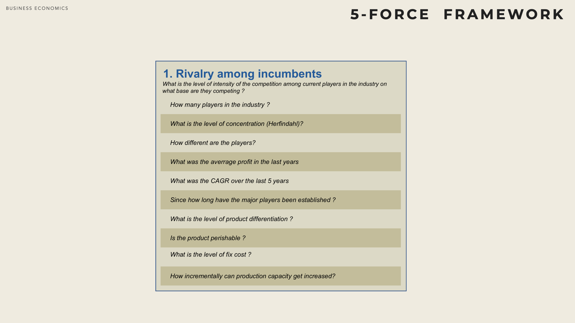
Five forces - Rivalry among incumbent players

Rivalry, the most obvious form of competition, can take many different forms: advertising campaigns, pricing, promotion and special offers, enhanced services, etc. How much rivalry impacts an industry’s profitability depends on the intensity with which firms compete but also on the basis on which they compete. Rivalry intensity is higher if:

• Many competitors usually increase rivalry. Indeed, establishing practices advantageous for the industry (as a whole) requires either a strong leader or a small group of competitors (oligopoly). Small number of players facilitate collusive behaviour (a collusive behaviour is a strategic anticipation and not an explicit agreements between firms - collusion- which is usually forbidden by antitrust laws). By contrast, the risk of war price increases with the number of similar players and/or when they all are of similar size and power.

• Competitor diversity measured by the degree of integration, diversification, geographical location etc. The more similar the players the more likely collusive behaviour. Conversely dissimilar firms are likely to seek to adopt more innovative and aggressive behaviour, which will impact industry profitability.

• Industry growth is limited (i.e.the industry is mature r declining). Players can only grow their market shares at the expense of the others (zero sum game). In non-mature markets, some players may also reduce unilaterally their prices and seek to capture big market share to be well positioned when the market gets mature.

• Exit barriers are high for instance there are specific assets or significant sunk costs – as firms can barely escape the industry, they will try to maintain themselves in the industry (in the hope of an economic recovery) as long as their losses are less than the exit costs. This usually creates overcapacity and drives price down for all players even the healthier.

• Some players have non-economic goals (e.g.image, employment, family owned business, CEO’s ego and prestige). Such high commitment to the business can lead to non-rational actions and decisions and become detrimental to the complete industry.

• Firms cannot read each other’s signal for instance due to a lack of familiarity with each other, cultural difference, unclear goals, diverse approaches to competing.

Rivalry can occur on various factors. However it is higher if it focuses on price only when:

• Little differentiation low customer loyalty (no brand value, the image or reputation of the vendor makes no difference), the products and/or services are perceived as equivalent (commoditisation: the goods are becoming simple commodities in the eyes of the consumers), buyers are facing little switching costs when changing providers.

• Fix costs are high and marginal costs are low volume becomes a major strategic parameter (economies of scale) and therefore all the players are tempted to reduce their price with the objective to i) capture more market share, ii) reduce their unit costs and iii) restore their long-term profit.

• Capacity must be expanded in large increments to avoid diseconomies of scale (e.g. new plant set-up). As a result, production increase far exceeds demand and overcapacity drives profitability down for the complete industry.

• Perishable product product that cannot get stocked (e.g.fresh vegetables) or goods that will soon get obsoleted (high tech products) or for which unsold capacity can’t be recovered (e.g. consultant or physician time, airline seat on a particular flight). Again, overcapacity will drive profitability down for all the players.

When competition apply on attributes other than price (e.g. enhance feature, better quality, complementary services), then the impact on industry profitability is more limited. Indeed, the enhancement usually translates into a higher perceived value which allows a price premium. It also raises entry barriers and reduces the threat of entry / threat of substitutes.

Rivalry among competitor relates to competition between firms that are already members of the industry. In large industry with many players, rivalry can be homogeneous (all players compete on similar attributes) or segmented (sub-groups compete on different attributes). To the extreme (perfect competition) no player can generate any profit in excess to its opportunity cost. In other words, the industry doesn’t generate any economic return.

Five forces - Threat to entry

Potential new entrants are firms that despite not being part of the industry yet, are threatening to enter and can be seen as latent players.

Incumbents have an incentive not to increase too much industry performance (i.e. their profit) as otherwise additional players will join and seek to grab market share, which would put pressure on price and elevate costs (e.g. increased R&D, marketing expenditure, etc).

Potential new entrants already established in other industries are even more threatening as they may leverage their existing capabilities and capital to shake up existing competition. Incumbents can deter new entrants by keeping their prices at rather lower levels and continuing to innovate and invest (which also reduce profit).

Competition authorities (anti-trust) consider that some markets (coined contestable markets by economists) are characterised by competitive equilibria despite being served by a very small number of players. In other words, the threat of entry is sufficient to cap profit (i.e. the part of value captured from customers).

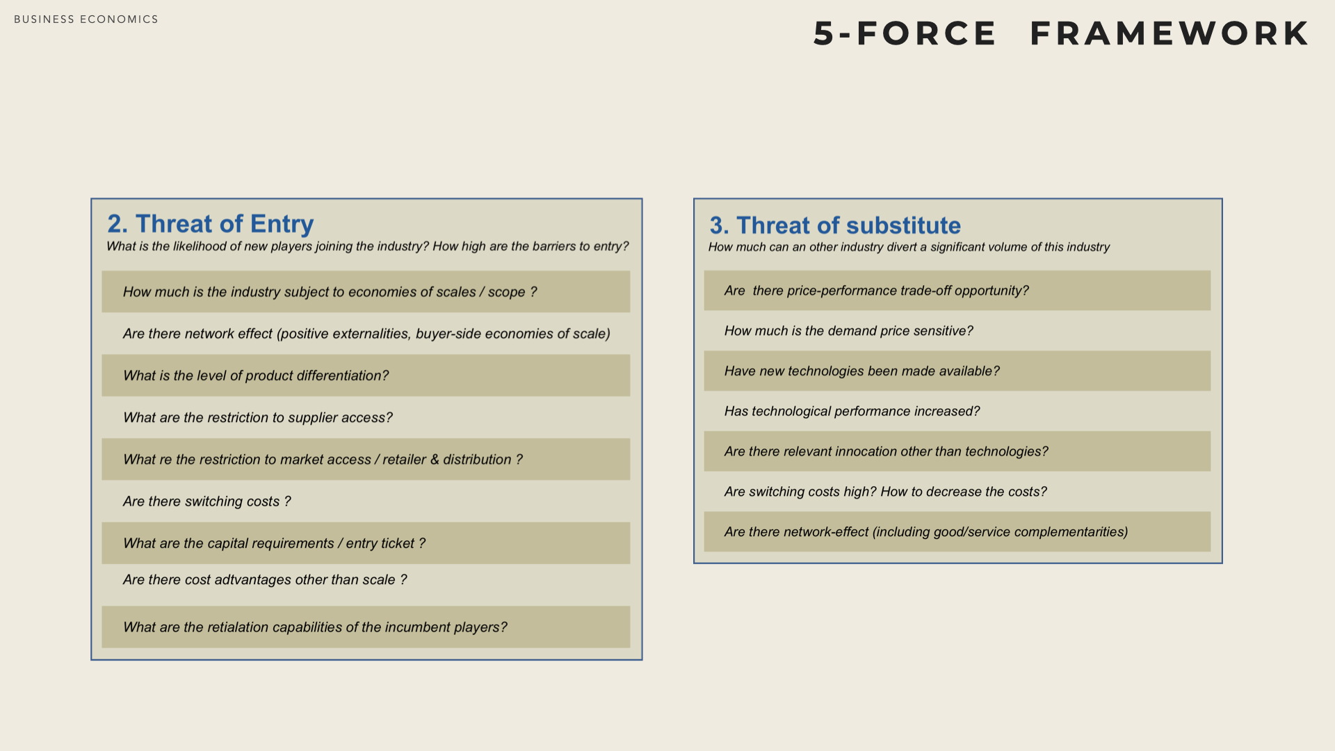
Barriers to entry increase with:

• Supplier-side economies of scale – firms that produce higher volume enjoy lower unit costs (fixed costs are averaged on more units, more efficient production processes & equipment, better terms & conditions from the supply base). A new entrant may either chose to produce a limited volume (and face far higher unit costs, which affects profit) or enter the industry directly with a large production volume (and experience significant overcapacity for a while).

• Network-effect (aka externalities, Buyer-side economies of scale) were the willingness to pay of buyers increase with the number of users of the good.

• Switching costs that a firm may incur (usually up-front, sunk costs) when moving from the installed supplier to a new one. This barrier is reduced for fast growing markets as incremental customer (i.e. new customers) don’t face switching cost.

• Investment needs to enter the industry (eg.fix assets: plants, equipment or working capital: inventory build up, customer credit or SG&A costs: development, advertising, etc) may be high. While large established firms may have both the willingness and financial capabilities to enter the industry, huge capital requirements is likely to reduce the number of prospective entrants. However, if the returns of the industry are attractive and are expected to remain so, potentially any new entrant can raise the funds from the capital market.

• Other cost advantage that incumbents may enjoy independently of their production volume (Ricardo rents). The may for instance, benefit from better access to key suppliers, protected patents, attractive geographic position, established brand recognition and reputation. In such a situation replicating the industry’s cost structure can be very challenging. However new entrant may decide to alter the current business model to counter the advantage of the entrenched players.

• Market access/distribution channels the more limited the wholesale or retail channels, the tougher the entry. Nevertheless, new entrant may decide to short-circuit existing distribution channels and create their own.

• Regulation and government policies can limit (e.g.licensing requirements, patents, intellectual property rights), forbid (e.g. restriction on foreign investment) or on the contrary, incentivise entries (subsidies, public R&D investments).

• Expected retaliation How incumbents would respond to a new player entering the industry can also be a barrier to entry, provided that incumbents are committed to defending their market and let it know (e.g. public statement, historical behaviour). The more available resources (e.g. cash) the stronger the resistance (war price, quality increase, advertising) and higher the entry barrier.

The threat of entry relates to the (potential) competition between a firm (the new entrant) and all incumbents players. If the threat materialises it impacts the market shares of entrenched players. High barriers to entry prevent additional players to join an industry. From the perspective of incumbents, barriers to entry protect the industry and protect profitability. Incumbents (especially in concentrated industries) will seek to in- crease barriers, for instance through contractual set-up (exclusivity, franchise, alliances) and lobbying actions.

«If entry barriers are low and new comers expect little retaliation from entrenched competitors, the threat of entry is high and industry profitability is therefore moderate» – [Porter, 2008b].

Incumbents will be particularly successful at strengthening entry barriers when:

• They can mobilise significant capital resources (cash, credit access)

• They are concentrated and can lock-in suppliers and customers

  • The industry is mature with low growth

Five forces - Threat of Substitutes

A substitute is a product or service that would be considered by customers as equivalent to the industry’s products. It has comparable functional attributes but is often based on different technologies (e.g. domestic flights vs. high-speed train, video rental shop vs internet video on demand).

Incumbents may fail to identify early enough substitutes, as they can be very different from the products currently offered by the industry (shop-around- the-corner vs amazon). An industry with little substitutes (rigid demand) is structurally more profitable.

Substitutes may emerge through technological innovations (e.g. wide deployment of the Internet), performance improvements of existing technologies (PC replacing mainframes), breakthroughs in cost structure, integration of various functions in a single product.

An industry will seek to reduce the threat of substitutes by lowering its own prices and/or increasing the product’s quality and features (so that customers will continue to prefer the industry’s product).

The threat of substitutes is higher if:

• Attractive price performance trade off can be offered, for instance through proposing different value-proposition (usually less sophisticated but much cheaper product) and increase the utility of some buyer groups.

• Low switching cost are associated with current products - i.e.there is little or no network-effect and customer loyalty is low.

• Price sensitive customers i.e. price-elasticity of demand is high - customers will tend to switch to any alternative, provided that price can be made more attractive.

«Every once in a while, a revolutionary product comes along, that changes everything. In 1984, Apple created the MacIntosh. It didn’t change only Apple, it changed the complete computer industry. In 2001, we introduced the iPod, it didn’t just changed the way we lis- ten to music, it changed the entire music industry. Today we are introducing three revolutionary products of this class. The first, is a widescreen iPod with touch control, the second a revolutionary mobile phone and the third is a breakthrough internet device. … An iPod, a phone and an internet communicator … these are not three separate devices, it is one device that we called an iPhone. Apple is going to revolutionise the Phone. » – Steve Jobs, 2007.

Five forces - Supplier / Buyer Power

These two forces depict how the participants that belong to the same value system (aka supply chain) can grab value. They have convergent interest in increasing the total created value, however they all seek to capture more of the value for themselves. This is clearly a zero sum game what one side wins, the other side looses.

If suppliers (including suppliers of labour usually represented by their unions) increase their transfer price, then industry profitability is likely to decline, except if industry participants can pass on the increase to their own customers. The reasoning that applies between suppliers and industry players, also applies between industry players and their customers.

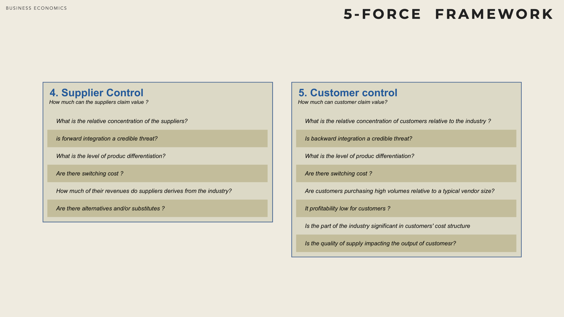
A supplier group is more powerful if:

• It is more concentrated than the industry is sells to (in other words, the most concentrated end has more power).

• It derives limited revenues from the industry and has a well balanced portfolio of customers. The more dependent of the industry the suppliers, the less market power.

• It offers highly differentiated products and/or services - commodisation on the contrary leads to reduced power.

• It can credibly integrate forward into the industry. Powerful customers can reduce industry profitability by driving prices down, requesting enhanced quality and/or services or playing industry participants

A customer group has more leverage if:

• They purchase high volumes relative to the size of a typical industry participant,

• Products are standardised and/or undifferentiated (commoditisation) or they enter into the production of an end-product and their quality has little impact on the quality of the end product. In such a situation buyers will face many potential suppliers, which highly increases their bargaining power. By contrast, if the inputs from a vendor are determinant (quality, performance, specific knowledge) then buyers will become less price sensitive and their willingness to pay will increase (until they find a substitute).

• Limited switching costs if any, when a customer changes its provider (transaction costs, transfer of work, risks).

• Integration threat Customers can credibly integrate backward into the industry

Customer groups will have incentives to use their market power if their profitability is low and/or they are suffering cash issues or if the product/service they procure:

• represents a significant part of their cost structure Buyers are more price-sensitive for the items that represent a high portion of their costs. By contrast, ’small items’ usually enjoy relatively better conditions.

• doesn’t impacts the quality of their own products Buyers view the product/service as a commodity and are ready to switch to a new supplier if necessary.

Market Power vs Negotiation Power

Market power is a characteristic of an industry as a whole (and applies equally to all players in that industry). It corresponds to the transfer of economic rents among the various stages of the production process (from raw material to end product). Market power reflects the ability of industry players to influence pricing mechanisms, raise price above marginal cost and earn a positive profit. Adopting collusive behaviour and/or limiting supply are typical behaviours that signal market power. Market power is also linked to the elasticity of the demand curve. By contrast to market power, negotiation power is specific to a given player (may vary across the various players of a same industry). It reflects the ability of the player to impose its preferences to its eco-system. For instance, large players will more easily obtain good conditions from their suppliers or retailers.

Additional Considerations about costs

Sunk costs, Avoidable costs

One of the key principle of micro-economics is that when a firm is facing a decision, past decisions cannot be undone and only that costs that the decision affects should be considered.

Sunk costs are those costs that are already incurred and cannot be recovered (not matter what). Once incurred they should be ignored in any future decision. Avoidable costs are those costs that can be recovered.

Ignoring sunk costs leads to a frequent fallacy. Assume that you launch the development of a product under the assumptions that it will cost 10 million. As you have already spent 8 million, a direct competitor unveils a similar product which cuts your addressable market by two. The 8 million already spent are sunk costs (assuming that what has been done cannot be re-used for any other purpose). So the decision to continue or stop should only be based on comparing the new market perspective with the 2 million investment that are still required to complete the development (and not the initial 10).

It is important to recognise that not all fixed costs are sunk costs. If you acquire an office building to host your headquarters you always have the option to re-sell it later (not necessarily at the same price though). By contrast, if you build rail tracks between two of your factories, it is very likely that associated investment are sunk costs.

Identifying Sunk costs is key to understand the structure of an industry and entry / exit decisions. More globally it is highly advisable to recognise before committing to any large expense what will be sunk cost and what will be avoidable cost.

Economic vs Accounting costs

Accounting tend to recognise three main types of costs: direct costs (aka Cost of Good Sold), indirect costs (aka Sales, General Management & Administration) and Amortisation & Depreciation.

Accounting statements such as the balance sheet and income statement are aimed at external audience (tax authorities, lenders, shareholders & investors). Accounting numbers are based on historical costs. For instance, to assess the value of an inventory of raw material, accounting will consider the (weighted average) price at which it has been purchased.

Business decisions (starting with strategy related decisions) however should be based on economic costs (i.e.take into account opportunity costs). In the example above, the value of an inventory is the price at which it could be sold on the market (regardless of the price at which it had been purchased by the firm).

We will see in the Value Equation section that to attract investors, a firm must generate a return that is at least as large as the return they could have received from the best investment of similar risk.

Price elasticity of demand

According to the law of demand (one of the most fundamental principle in micro-economics) the overall quantity of a good that consumers are ready to buy is a function of the price of the good. The higher the price the less quantity is sold.

When a firm changes its pricing policy (for instance increases the price) it will impact its addressable market (for instance sell less), its average cost and its profit. While this principle applies to all industries the magnitude of the effect is highly variable from one good to the next (and depends usually as well on the level output).

The elasticity of demand measures the sensitivity of the effect. It is defined as the variation of demand relatively to the variation of price.

\[ \epsilon = - \frac{\frac{dq}{q}}{\frac{dP(q)}{P(q)}}\]

If \( \epsilon \) is less than 1, the demand is inelastic. A classical example is fuel (gasoline) with elasticity around 0.1 to 0.2 - which means that even when fuel price double, the total quantity is reduced by around 30%. At the extreme when \( \epsilon \) is null, the demand is totally inelastic (the quantity sold remains identical no matter the price level).

If \( \epsilon \) is more than 1, the demand is elastic.

Price elasticity can be assessed numerically (that typically what econometrics an do). Qualitatively a product is more price-sensitive (elastic) when i) differentiation compared is limited and competitors’ price are easily accessible, ii) the price of the product represents a large chunk of the buyer’s expenditure or budget. Conversely a product is less elastic when i) comparison among competing or substitute products is difficult or costly, ii) switching costs are high, iii) the product is a complement to an other product that has very high switching costs.

In a highly competitive market, if one firm only changes their price (and their rivals don’t match that new price) then it is likely that most of the demand will shift to the firms with the lowest price.

In a situation of perfect competition, a firm has no impact on the market price (firms are price takers) and the demand curve that see each firm is constant (an horizontal line at the market price \( P = P^* \)). In that case price elasticity is infinite.

TOTAL and MARGINAL REVENUE

The total revenue function of a firm denotes the revenue captured by the firm as a function of its level of production \( q \). The total revenue equals the quantity times the price for that quantity (demand curve).

\[R(q) = P(q) * q \]

The marginal revenue is the derivative of the total revenue function and represent the addition revenue derived from selling one additional unit.

\[ \frac{dR(q)}{dq} = \frac{dP(q)}{dq} * q + P(q) = P(q) * [ \frac{dP(q)}{P}* \frac{q}{dq} + 1 ] \] \[ \frac{dR(q)}{dq} = P(q) * ( 1 - \frac{1}{\epsilon} ) \]

It follows that if demand is inelastic, ( i.e \( \epsilon \) is less than 1) then \( \frac{1}{\epsilon} \) is more than 1, which entails that \( ( 1 - \frac{1}{\epsilon} ) \) is negative and therefore the total revenue decreases.